AC and TRAN tutorial
While the simulation below might me done from the command line with an netlist file, interacting with the simulator inside a Python program gives the user the ability to employ all the extreme flexibility and power of the Python language.
This page gives an beginners tutorial showing how, especially illustrating AC
and TRAN simulations. Please refer to the doc pages for ahkab and
ahkab.circuit for more.
Tutorial
Let’s say we would like to simulate the AC characteristics and the step response of a Butterworth low pass filter, such as this:
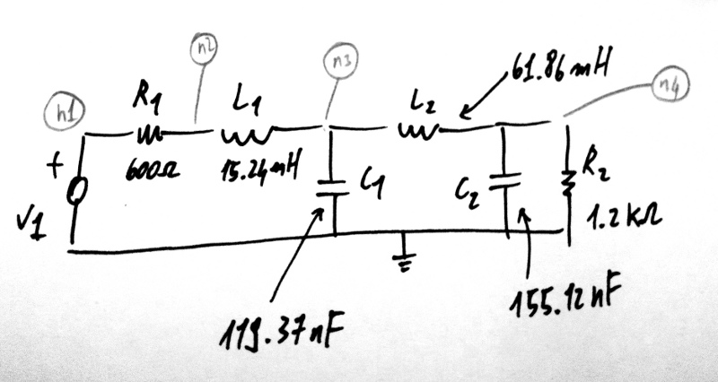
This example is example 7.4 in from Hercules G. Dimopoulos, Analog Electronic Filters: Theory, Design and Synthesis, Springer.
The code to describe the circuit is the following:
First import the modules and create a new circuit:
import ahkab
from ahkab import circuit, printing, time_functions

mycircuit = circuit.Circuit(title="Butterworth Example circuit")
Elements are to be connected to nodes. There is one special node, the reference (gnd):
import ahkab
from ahkab import circuit, printing, time_functions
mycircuit = circuit.Circuit(title="Butterworth Example circuit")

gnd = mycircuit.get_ground_node()
and ordinary nodes.
Ordinary nodes can be defined as:
# setup
import ahkab
from ahkab import circuit, printing, time_functions
mycircuit = circuit.Circuit(title="Butterworth Example circuit")
# now we can define the nodes
# 1. using arbitrary strings to describe the nodes
# eg:
n1 = 'n1'
# 2. using the alternative syntax:
n1 = mycircuit.create_node('n1')
# the helper function create_node() will check that this is not a
# node name that was used somewhere else in your circuit
Then you can use the nodes you have defined to add your elements to the circuit. The circuit instance provides convenient helper functions.
The passives in example 7.4 can be added as:
import ahkab
from ahkab import circuit, printing, time_functions
mycircuit = circuit.Circuit(title="Butterworth Example circuit")

gnd = mycircuit.get_ground_node()

mycircuit.add_resistor("R1", n1="n1", n2="n2", value=600)
mycircuit.add_inductor("L1", n1="n2", n2="n3", value=15.24e-3)
mycircuit.add_capacitor("C1", n1="n3", n2=gnd, value=119.37e-9)
mycircuit.add_inductor("L2", n1="n3", n2="n4", value=61.86e-3)
mycircuit.add_capacitor("C2", n1="n4", n2=gnd, value=155.12e-9)
mycircuit.add_resistor("R2", n1="n4", n2=gnd, value=1.2e3)
Next, we want to add the voltage source V1.
- First, we define a pulse function to provide the time-variable characteristics of V1, to be used in the transient simulation:
voltage_step = time_functions.pulse(v1=0, v2=1, td=500e-9, tr=1e-12, pw=1, tf=1e-12, per=2)
- Then we add a voltage source named V1 to the circuit, with the time-function we have just built:
mycircuit.add_vsource("V1", n1="n1", n2=gnd, dc_value=5, ac_value=1, function=voltage_step)
Putting all together:
voltage_step = time_functions.pulse(v1=0, v2=1, td=500e-9, tr=1e-12, pw=1, tf=1e-12, per=2)
mycircuit.add_vsource("V1", n1="n1", n2=gnd, dc_value=5, ac_value=1, function=voltage_step)
We can now check that the circuit is defined as we intended, generating a netlist.
print mycircuit
If you invoke python now, you should get an output like this:
* TITLE: Butterworth Example circuit
R1 n1 n2 600
L1 n2 n3 0.01524
C1 n3 0 1.1937e-07
L2 n3 n4 0.06186
C2 n4 0 1.5512e-07
R2 n4 0 1200.0
V1 n1 0 type=vdc vdc=5 vac=1 arg=0 type=pulse v1=0 v2=1 td=5e-07 per=2 tr=1e-12 tf=1e-12 pw=1
Next, we need to define the analyses to be carried out:
op_analysis = ahkab.new_op()
ac_analysis = ahkab.new_ac(start=1e3, stop=1e5, points=100)
tran_analysis = ahkab.new_tran(tstart=0, tstop=1.2e-3, tstep=1e-6, x0=None)
Next, we run the simulation:
r = ahkab.run(mycircuit, an_list=[op_analysis, ac_analysis, tran_analysis])
Save the script to a file and start python in interactive model with:
python -i script.py
All results were saved in a variable ‘r’. Let’s take a look at the OP results:
>>> r
`{'ac': <results.ac_solution instance at 0xb57e4ec>,
'op': <results.op_solution instance at 0xb57e4cc>,
'tran': <results.tran_solution instance at 0xb57e4fc>}`

>>> r['op'].results
{'VN4': 3.3333333333333335, 'VN3': 3.3333333333333335, 'VN2': 3.3333333333333335,
'I(L1)': 0.0027777777777777779, 'I(V1)': -0.0027777777777777779, 'I(L2)': 0.0027777777777777779, 'VN1': 5.0}
You can get all the available variables calling the keys() method:
>>> r['op'].keys()
['VN1', 'VN2', 'VN3', 'VN4', 'I(L1)', 'I(L2)', 'I(V1)']
>>> r['op']['VN4']
3.3333333333333335
Then you can access the data through the dictionary interface, eg:
>>> "The DC output voltage is %s %s" % (r['op']['VN4'] , r['op'].units['VN4'])
'The DC output voltage is 3.33333333333 V'
A similar interface is available for the AC simulation results:
>>> print(r['ac'])
<AC simulation results for Butterworth Example circuit (netlist None).
LOG sweep, from 1000 Hz to 100000 Hz, 100 points. Run on 2011-12-19 17:24:29>
>>> r['ac'].keys()
['#w', '|Vn1|', 'arg(Vn1)', '|Vn2|', 'arg(Vn2)', '|Vn3|', 'arg(Vn3)', '|Vn4|',
'arg(Vn4)', '|I(L1)|', 'arg(I(L1))', '|I(L2)|', 'arg(I(L2))', '|I(V1)|', 'arg(I(V1))']
And a similar approach can be used to access the TRAN data set.
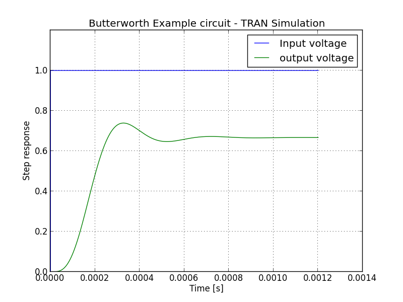
The data can be plotted through matplotlib, for example:
import pylab as plt
import numpy as np
fig = plt.figure()
plt.title(mycircuit.title + " - TRAN Simulation")
plt.plot(r['tran']['T'], r['tran']['VN1'], label="Input voltage")
plt.hold(True)
plt.plot(r['tran']['T'], r['tran']['VN4'], label="output voltage")
plt.legend()
plt.hold(False)
plt.grid(True)
plt.ylim([0,1.2])
plt.ylabel('Step response')
plt.xlabel('Time [s]')
fig.savefig('tran_plot.png')
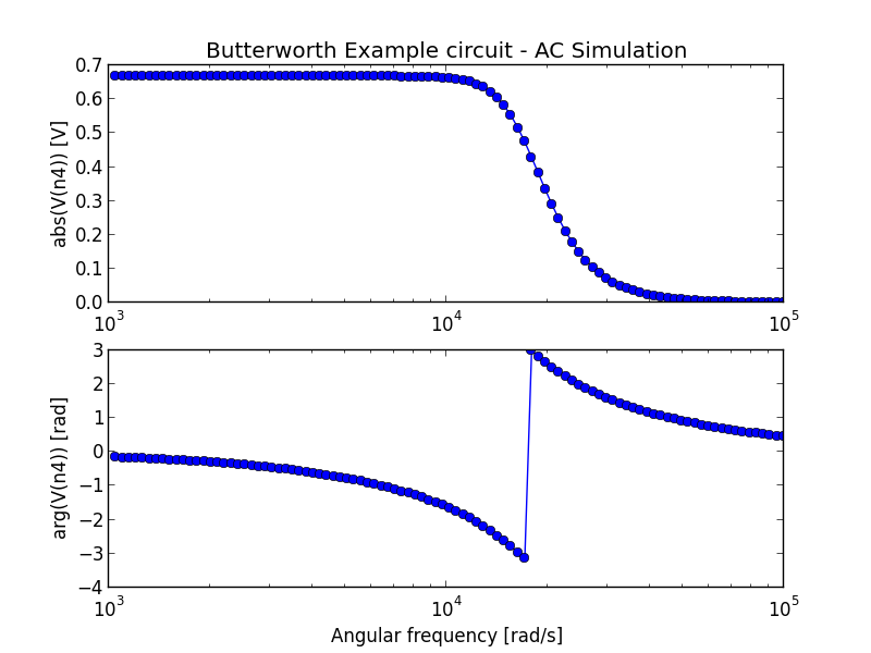
fig = plt.figure()
plt.subplot(211)
plt.semilogx(r['ac']['w'], np.abs(r['ac']['Vn4']), 'o-')
plt.ylabel('abs(V(n4)) [V]')
plt.title(mycircuit.title + " - AC Simulation")
plt.subplot(212)
plt.grid(True)
plt.semilogx(r['ac']['w'], np.angle(r['ac']['Vn4']), 'o-')
plt.xlabel('Angular frequency [rad/s]')
plt.ylabel('arg(V(n4)) [rad]')
fig.savefig('ac_plot.png')
plt.show()
The previous code generates the following plots:
It is also possible to extract attenuation in pass-band (0-2kHz) and stop-band (6.5kHz and up).
The problem is that the voltages/currents we are looking for may not have been evaluated by ahkab at the desired points. This can be easily overcome with interpolation through scipy.
Here is a snippet of code to evaluate the attenuation is pass-band and stop band in the example:
import numpy as np
import scipy, scipy.interpolate

# Normalize the output to the low frequency value and convert to array
norm_out = np.abs(r['ac']['Vn4'])/np.abs(r['ac']['Vn4']).max()
# Convert to dB
norm_out_db = 20*np.log10(norm_out)
# Convert angular frequencies to Hz and convert matrix to array
frequencies = r['ac']['w']/2/np.pi
# call scipy to interpolate
norm_out_db_interpolated = scipy.interpolate.interp1d(frequencies, norm_out_db)

print "Maximum attenuation in the pass band (0-%g Hz) is %g dB" % \
(2e3, -1.0*norm_out_db_interpolated(2e3))
print "Minimum attenuation in the stop band (%g Hz - Inf) is %g dB" % \
(6.5e3, -1.0*norm_out_db_interpolated(6.5e3))
You should see the following output:
Maximum attenuation in the pass band (0-2000 Hz) is 0.351373 dB
Minimum attenuation in the stop band (6500 Hz - Inf) is 30.2088 dB
